Procurement plan and regulatory costs. Adjustments to price series using moving averages
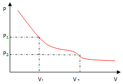
The need for adjustments is not necessarily related to the modeling of external risks. For example, forecast prices were based on forecasts of wholesale prices, more volatile than prices at subsequent stages in the sales chain.
Budget-Plan Express is a software product for preparing business plans and presentations in Word and Excel format, optimal for small businesses and studies (for students, graduate students, MBI students, etc.)
Build a financial model of your project or calculate loan financing on different terms! Try the new version of the program (6.02). Details ...
In the first case you can use method of correcting price fluctuations mathematically "describe" the possible influence of factors external risks. In the second case can be useful method of smoothing short-term fluctuations.
In the first and in the second case used models moving averages.
Selecting a model and adjusting the parameters of moving averages
In the settings menu options moving averages you can choose one of 3 models moving averages and configure the appropriate settings.
 Menu "Model settings."
- Selecting the Moving Average Model (SMA, WMA, and EMA)
- Smoothing interval (3-6)
- Forecast interval (1-3)
- Smoothing Constant (0.1-1.0)

 "Smoothing interval" is only set for SMA and WMA models (non-exponential models), while "Smoothing Constant" is only for EMA.
Default values:
- Selecting a Moving Average Model: SMA
- Smoothing interval: 3
- Forecasting interval: 1
- Smoothing constant: 0.5
 Menu "Construction of moving averages".
- The price forecast for the specified interval ...
- Smoothing the price range ...
- Save data (Save current values / Restore old values)

The method of adjusting price fluctuations
The method of adjusting price fluctuations (seasonal adjustment) is used to adjust for unexpected price changes associated with sudden changes in external factors that affect the level of price ranges. The definition of possible risks of price fluctuations (as a rule, short-term jumps) is especially important with a high degree of price elasticity of demand for a price.
The method of adjusting price fluctuations is used for a high degree of correlation between external factors and price formation (the factor's influence on the price). The calculation is not related to finding the correlation coefficient, the correlation should be sufficient (according to expert judgment) to include this factor in the calculation of risk planning.
The level of correlation, in general, is determined by expert estimates. For example, if you sell medicines that are not manufactured in Russia, then the price directly depends on fluctuations in the exchange rates. In this case, the risk factors are unfavorable changes in the exchange rate trend, and in the calculations these risks will be taken into account - as a correlating trend (a trend correlating with price quotes).
Another example. The company is engaged in transportation, another company is engaged in the production of agricultural products. In one and the other case, the risk factor (a correlating trend) is the price of gasoline or diesel fuel. In other words, the initial price of the product is in varying degrees dependent on the forecast trends.
Forecasting trends
To external factors can be attributed as the change in energy prices and other forecasted trends related to total risk – inflation, the key rate of the Central Bank of the Russian Federation, other rates and indexes. To use in pricing calculations correlating trends, those trends must first be created. Budget-Plan Express can be used five predictive trends (any external risk factors) and trends in exchange rates, which are equally factors external risks. How to plan for trends, see "Forecasting trends. Forecast exchange rates".
The method adjustments to the price fluctuations
To detect sharp jumps (in the forecast trend), the "standard deviation" is used (the indicator of scattering the values of a random variable relative to its mathematical expectation) from the moving average. The algorithm uses parameters and models of user settings of the moving average, installed by the user. Correction of price fluctuations for a certain period, using the standard deviation, allows you to respond to fluctuations in the trend and "ignore" trend changes within the standard deviation.
Example.
Suppose the price of goods depends on changes in the dollar. In trends, the forecasted dollar rate for the first year is as follows:
Coursei = {67,64 66,92 66,20 65,00 64,76 64,04 63,32 62,60 61,88 61,16 60,44 59,00}.
Let the expected average annual price is "200", projected seasonal price fluctuations (in%):
Аi = {0% 4% -1% 3% 2% -2% 2% 3% 2% -1% -4% 4%}.
In the "Model settings" (form menu) - default settings:
- Selecting a Moving Average Model - SMA -simple moving average
- Smoothing interval - 3
It is necessary to perform the price calculation taking into account the jump in the dollar exchange rate in the 4th month to the level 90,00.
Step-by-step actions:
- step . Go to the "Financial analysis" page and set the dollar rate in the 4th month 90,00 , instead of 65,00.
- step . Let's go to the product planning form and set the price to 200 for the entire period.
- step . Set the seasonality values.
- step . "Calculate" button → "interpolation of the series on the trend":
- step . Press the button "Correlating trend" → "Dollar rate" → "OK":
- step . The calculation can be saved, or you can restore the old values: "Construction of moving averages" → "Save data" → "Save (restore) current values"
| Periods | Jan | Feb | March | Apr | May | June | July | Aug | Sen | Oct | Nov | Dec |
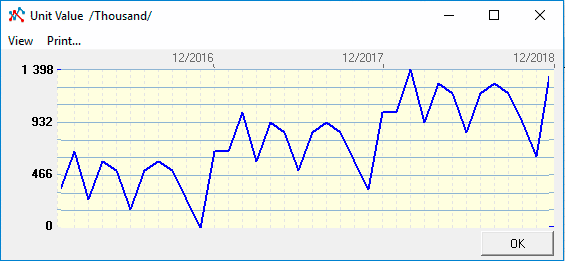
| Result of calculation of the price for 1 year | 200 | 208 | 198 | 206 | 204 | 196 | 204 | 206 | 204 | 198 | 192 | 208 |
| Periods | Jan | Feb | March | Apr | May | June | July | Aug | Sen | Oct | Nov | Dec |
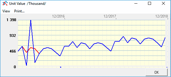
| Result of calculation of the price for 1 year | 200 | 208 | 176 | 252 | 181 | 196 | 204 | 206 | 204 | 198 | 192 | 208 |
To create a price chart, select the line "price" (click on the row name), right-click to open the context menu ...
Graphs of the price trend after the calculation step 4:
Graphs of the price trend after the calculation step 5:
 It is important to understand that the result of the calculation affects not only the volatility of the trend and the settings of the moving averages models.
 In order to take into account the inertia of the influence of external factors, the trend must be shifted for several periods ahead.
Method of smoothing short-term fluctuations
In the "Budget-Plan Express" three basic models of sliding SMA (simple moving average), WMA (weighted moving average) and EMA (exponential moving average) are used. To modify the series, any models can be selected, depending on the type of calculations and data. Before starting calculations, using the smoothing method, you need to set the settings with the menu option, as described above, then select the menu item: "Construction of moving averages" → "Smoothing range of price". The result of the modification of the series can be seen on the graph.
Example.
Let the forecast of average annual wholesale prices for the following product: the Price of = 200, projected seasonal price fluctuations (in %):
Аi = {0% 5% -2% 2% -7% 6% 1% -4% -7% 2% 5% 3%}.
In the example, to smooth the series, we use the model EMA with a smoothing constant 0.5.
Step-by-step actions:
- step . In the product planning form: 1) set the "Price forecast" switch, 2) set the price 200 for the entire period.
- step . Set the seasonality values.
- step . "Calculate" button → "interpolation of the series on the trend":
- step . Install the EMA model in the settings menu: "Settings for model parameters" → "Selecting a Moving Average Model" → EMA
- step . Set the anti-aliasing constant for EMA in the settings menu: "Settings of model parameters" → "Smoothing constant" → 0.5
- step . Let's execute calculation: "Construction of moving averages" → "Smoothing a price range" .
- step . Save data: "Construction of moving averages" → "Save current values" . Pay attention, the initial values of the series (calculation of 36 months) were in the range: 186-225, after smoothing the oscillations of the series - in the range: 192-218.
The result of the calculation is presented on the graph:
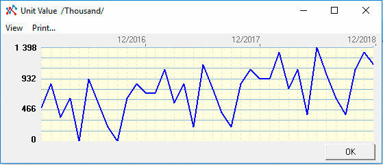
To create a chart, select the line "price" (click the mouse on the line name) and call the context menu.
The result of the calculation is presented on the graph:
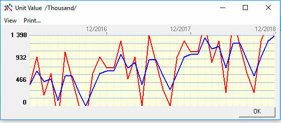
Note that two graphs appeared: a graph with new values and a graph with old values.
 For EMA , the sensitivity depends on the coefficient - a: for a → 1 , the values of EMA t → to the values of the original series , and vice versa: with a → 0 , values of EMA t → to the values of the midline of the row .
The result, once saved, are represented on the chart:
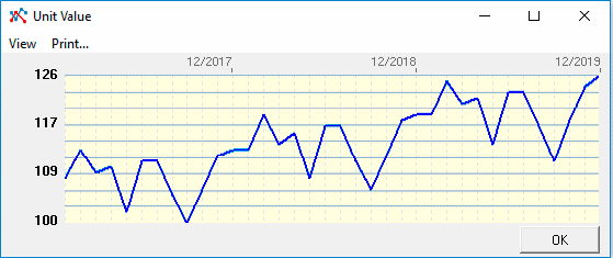
Table of calculation results for 1 year:
| Periods | Jan | Feb | March | Apr | May | June | July | Aug | Sen | Oct | Nov | Dec |
| Old values - pricing 1 year | 200 | 210 | 196 | 204 | 186 | 212 | 202 | 192 | 186 | 204 | 210 | 206 |
| New value - pricing 1 year | 200 | 205 | 201 | 202 | 194 | 203 | 203 | 197 | 192 | 198 | 204 | 205 |
| Delta - the difference between the old and new values | 0 | 5 | -5 | 2 | -8 | 9 | -1 | -5 | -6 | 6 | 6 | 1 |
Short-term forecasts based on moving average models
Before you start building a short-term forecast, based on moving average models, you need to set the menu settings as described above, then select the menu item: "Construction of moving averages" → "Forecast prices for the specified interval". The result of the modification of the series can be seen on the graph.
Example.
Let the forecast of average annual wholesale prices for the following product: the Price of = 200, projected seasonal price fluctuations (in %):
Аi = {0% 5% -2% 2% -7% 6% 1% -4% -7% 2% 5% 3%}.
Task. To build a short-term forecast for the end of 2015 beginning of 2016: 10.2015-03.2016. In the example, to build a short-term forecast of the series, we use a simple moving average model - SMA with a forecast interval of 3.
Step-by-step actions:
- step . Let's go to the product planning form and set the price "200" for the whole period.
- step . Set the seasonality values.
- step . "Calculate" button → "interpolation of the series on the trend":
- step . Install the SMA model in the settings menu: "Settings of model parameters" → "Selecting a Moving Average Model" → SMA.
- step . We set in the settings menu Forecasting interval: "Settings of model parameters" → "Forecasting interval" → 3.
- step . Set the calculation start period: "10.2015" .
- step . Perform the calculation: "Construction of moving averages" → "Forecast prices for the specified interval". The number of the calculated periods ≡ N + 1.
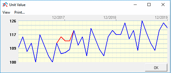
Result of calculation on the graph:
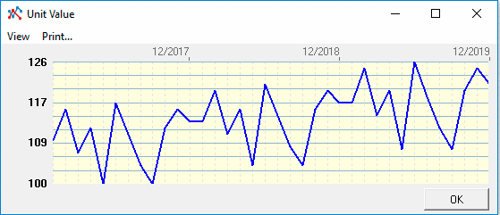
To create a chart, select the line "price" (click the mouse on the line name) and call the context menu (right mouse button).
 To construct a short-term forecast, at least three observation periods are required, not including the current period. If the calculation period is not set correctly, the program will display an error message.
The program calculates and displays the following message on screen:
-
[Set forecast values?
Period: 01.2016 (194) 03.2016 (195) 03.2016 (198)]
Result of calculation on the graph:
