In this case, just enter their values using normal editing, or enter a value in the initial period, then right-click (above the value field) and select "continue trend" from the menu, and the current value will be set - to the end of the series. You can change the value of the series in any period and perform the function "continue the trend", starting from this period.
Sales plan. Practical planning
Sales planning algorithm
For the fastest and most reliable sales planning, the program has created special tools for planning and adjusting prices and sales volumes of any complexity, including in the face of changing external factors.

Budget-Plan Express is a software product for preparing business plans and presentations in Word and Excel format, optimal for small businesses and studies (for students, graduate students, MBI students, etc.)
Build a financial model, calculate the options for sales plans of any complexity yourself! Try the new version of the program (6.02). Details ...
☛ Important! An additional conditional future period has been added to all plans. However, only in the plans of loan and rental products can you plan with an estimated horizon of up to 10 years (up to 120 months). At the same time, all calculations - outside the standard horizon - will be taken into account in the conditional future period. That is, the future period will accumulate all the calculations that will go beyond the 36 months of the project.
Step 1. Planning the price and quantity (sales volumes). Sales planning table tab
Planning Algorithm 1. If you have static (unchanging, rarely changing) prices and sales volumes
Planning algorithm 2. Planning, adjusted for seasonal fluctuations (interpolation of the forecast series)
1. First, as in Algorithm 1, the initial fields in the price and quantity rows are filled in, then the row is filled in (“continue trend” function). Please note that the "continue trend" function can be used starting from any new period (for example, a year).
2. Then edit the forecast trends - prices and sales volumes using the sliders. Values from -100 to +100 are available for the price, i.e., relative price changes (%) from the initial (beginning of the year). Values from 0 to +100 are available for sales volumes, i.e. relative seasonal changes in sales volumes (%) of the maximum value (100%). To see the values of the slider - move the mouse to the slider. Use the arrows (for the active slider) to set the exact value.

3. Finally, perform the price and sales calculations in sequence. To calculate the price, select the "price" option, click the "Calculate" button, in the question form "What to calculate?" select the 2nd item "Adjust the 'Price' series using interpolation of the forecast series". Click OK.
Also, to calculate sales volumes, select the "sales volume" option, click the "Calculate" button. Also select the 2nd item, now you will see the following title "Adjust the 'Quantity' series using interpolation of the seasonality series" Click "OK".
Thus, you filled the series and adjusted the series values using forecast series interpolation.
Planning algorithm 3. Planning by annual values, adjusted for seasonal values and forecast dynamics of price changes
This is the fastest and, perhaps, the most correct way of planning sales, since all calculations in this way are "tied" to annual values. And, as a rule, marketing forecasts, when assessing prices, sales volumes, when assessing external risks, are almost always calculated and guided, at least, for the next year.
1. So, first select the "price" option, and at the beginning of each year, enter the price in the fields. Then, similarly, use the sliders to adjust the forecast trend “Forecast of the annual price change”.
2. Then select the Sales Volume option, and for each year enter the annual (for the entire year) sales volume. Then, similarly, adjust the forecast trend “Sales forecast (seasonality)” using the sliders.
3. Finally, do the final calculation of the sales plan. Press the button "Calculate", in the form select the 1st item "Calculate 'Price' and 'Quantity' using annual values and forecast series." Click OK.
Thus, in this case, annual values and forecast series were used. In this case, one calculation was performed for the entire sales plan (for price and quantity).
☛ Any of the calculation methods will take no more than 1-2 minutes. When choosing a calculation method, it is important that the sales plan is the most reliable, based on the most authoritative expert assessments and forecasts. As a rule, annual forecasts are considered the most accurate, as they take into account a combination of external and other risks.
Step 2. Further price adjustments
In order to most accurately adjust prices, taking into account external and other factors, the program has powerful tools to support complex calculation methods. Moving average models are used for such calculations. For detailed information on these methods, see the Help topics "Adjusting Price Series Using Moving Average" and "Moving Average Model". Also (recommended) watch a video with a detailed explanation of the calculations using these methods (see Lesson 4. Parts 3, 4).
Step 3. Accounting for safety stock
Before making the final calculations, if necessary, you can take into account the limit level of the safety stock as a percentage. It must be specified as a percentage in the tab "accounting for stocks of finished goods". The data in the table "balances of finished products at the beginning of the period" will appear only after the final calculation has been completed.
Step 4. Calculation of the sales plan table for this product
So, all the calculations of the sales plan for this product are still in the "edit sales" form. When you are sure that these calculations are final, you can perform the following calculation, after which the sales plan (for this product) will appear in the final sales table, along with other products. Click the "Calculate" button and select "Calculate the sales plan table for this product." Click OK.
Step 5. Final calculation of the sales plan
After all the sales plans for all products are ready, you need to do the final calculation. After this calculation, the sales plan will be included in the calculation structure of the business plan. Select in the tab of the main menu “data” the menu item “calculate” or press F9. In the form that opens, select the appropriate plan, in this case, the sales plan (Data → Calculate → “Sales plan”. Same thing - F9).
And after performing the calculation, in addition, taxes (VAT, if it is taken into account), safety stock and other parameters will be calculated, which will be used in the future when calculating the business plan. Now you can go to the form for editing the sales of any product, and you will see the calculated tax (VAT, if it is taken into account) and the safety stock.
How to calculate the seasonality trend
Seasonality trend table example
| Sales volume for the last year | Jan | Feb | Mar | Apr | May | Jun | Jul | Aug | Sep | Oct | Nov | Dec |
| Sales volume for the period | 1 500 | 1 350 | 1 200 | 1 200 | 900 | 600 | 600 | 600 | 900 | 1 050 | 1 200 | 1 350 |
| Trend of seasonality (100 points scale) | 100 | 90 | 80 | 80 | 60 | 40 | 40 | 40 | 60 | 70 | 80 | 90 |
To calculate the seasonality trend (for example, on a 100-point scale), take the sales trend for the last year (or the weighted average trend over the past few years). Then, in the line where we calculate the seasonality values, opposite the maximum value of the sales volume (this can be several values), put the number 100 (in this example, the maximum value in January). To calculate the values in other cells, you need to divide the value of the current cell by the maximum and multiply by 100. And so - for each cell, for example:
- Seasonality factor for February = 1350 / 1500 * 100 = 90
- Seasonality factor for March = 1200 / 1500 * 100 = 80 Etc.
☛ Note, if you want to build a seasonal trend, for example, on a 10-point scale, then multiply it by 10, respectively.
Special tool - slider
To adjust the values of seasonality, use a special tool - the slider. The admissible values are from "0" to "+100" (when planning sales volumes) and from "-100" to "+100" (when planning prices). The sliders edit the seasonality values (monthly values in percent) during the annual cycle (12 months).
The values of the slider can be set with the mouse or the arrow keys (preliminary, activate the slider, hover the mouse, as shown in the picture).
Button Assignment
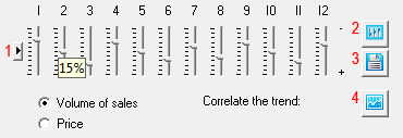
1. To set default values.
All periods of seasonality relating to sales by default are set to "100", and is related to price – value "0".
This is due, first of all, to the specifics of calculating trends in sales volumes and prices: prices are calculated as deviations from a given value.
2. Download trend settings from other products.
3. To save values.
4. Correlation trend.
Planning methods

Go to the "Sales plan", select the product and call the editing form.
"sales Planning" (one click with the left mouse button, same F2):
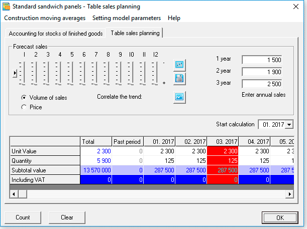
In the form of "Sales planning", start planning sales of the product in one of the ways:
1 way. "Continue trend" function
Use the "continue trend" function if the price for a product changes not so often, for example, every six months. This is the easiest and fastest way to fill a series of prices with a trend.
- step. Enter the value in the cell where planning begins.
- step. Click the right mouse button (above the cell), and select "continue trend". As a result of the function, the series will be filled to the end.
- step. Select the next period when you want to set a new price. Do step 1,2 - from any subsequent period ...
The result of the "Continue trend" function:


2 way. Function "interpolation of the series by trend"
Function "interpolation of the series by trend" Use the function "interpolation of the series by trend", if you already have a filled series and you need to interpolate the values of this series in the seasonal trend.
☛ Note that the function is called when the series already exists when the "Calculate" button is pressed.
- step. Enter the data using the "continue trend" function.
- step. If necessary, set the calculation start period.
- step. Click the "Calculate" button and select "interpolate the series by trend". As a result, the series will be filled to the end, taking into account seasonality factors.
 Steps 1-3 are performed separately - for planning either a price or an amount.
Example . Application of the function "interpolation of the series by trend"
Set a product price, "100", starting from the first month of the project,
as shown in the figure below:

Let, target price will increase by 7% in 5-m and 10-m month. Install the appropriate values (in 5-m and 10-m month) in the seasonality trend of prices as shown in the figure below:
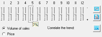
Click "Calculate" and execute point 2: "interpolation of the series by trend". As a result of executing, all the data of a number of prices, starting with 5-th and 10-th month, will increase by 7%.
Data of the calculation result are shown in table:
| Interpolation of a number of the trend - years | Jan | Feb | March | Apr | May | June | July | AVG | sen | Oct | Nov | Dec |
| 1 year. Price changes in 5 and 10 month | 100 | 100 | 100 | 100 | 107 | 107 | 107 | 107 | 107 | 114 | 114 | 114 |
| 2 year. Price changes in 5 and 10 month | 114 | 114 | 114 | 114 | 122 | 122 | 122 | 122 | 122 | 130 | 130 | 130 |
| 3 year. Price changes in 5 and 10 month | 130 | 130 | 130 | 130 | 139 | 139 | 139 | 139 | 139 | 148 | 148 | 148 |
 When using "series interpolation by trend", new values (prices or quantities) are calculated relative to the old values, taking into account the seasonality factors. When calculating this method, an identical algorithm is used - to calculate sales volumes and prices.
3 way. Sales planning "by yearly values"
Use the function "by annual values" for sales planning if you have the following sales parameters: for sales volumes - seasonality of demand and annual sales, for prices - seasonality of price fluctuations and prices for the beginning of the year.
☛ Note that the function is called when the series already exists when the "Calculate" button is pressed.
- step. Enter the annual sales volume (quantity), respectively, for 1,2 and 3 year.
- step. Adjust the seasonal factors of sales on a 100-point scale (from 0-100).
- step. Set the "Price forecast" switch and enter the prices for the beginning of the year, respectively, for 1,2 and 3 yeara.
- step. Adjust the seasonal price coefficients (from -100% to 100%).
- step. Click the "Calculate" button and select "Sales plan - by yearly values" .
Example. Consider a simple example of planning a cyclical sales plan for a contingent product. According to the forecasts of marketing expert estimates, when analyzing the regional market, the parameters of sales are determined: for sales volumes - seasonality and annual sales volumes (for 3 subsequent years), for prices - seasonality of price fluctuations and prices at the beginning of the year. That is, the marketing department prepared a table of seasonality factors (based on seasonality factors for past periods) and probabilistic estimates of annual sales volumes of product N::
- for 1 year - 10,000 units,
- for 2 yeara - 12,000 units,
- for 3 years - 15 000 units
Table shows the seasonal demand factors (sales volumes), in percentages:
| Months | 1 | 2 | 3 | 4 | 5 | 6 | 7 | 8 | 9 | 10 | 11 | 12 |
| Coefficients | 100 | 90 | 80 | 80 | 60 | 40 | 40 | 40 | 60 | 70 | 80 | 90 |
As can be seen from the table that maximum sales are during the winter months, minimum in summer. When planning sales, you always need to consider probabilistic seasonal cycles predicted by taking into account observations of past and current changes in market conditions.
In addition, it is assumed that the first 3 months the company will be able to realize no more than 50% of the planned volume of sales, the next 2 months – not more than 70%, then 100% of the target sales.
The price of product N, to simplify the example, will be considered without VAT. Let the initial price of the product 100. Suppose that every six months (in the 1st and 6th months) the price will increase by 5%.
To plan the sales of product N, in the form of planning, follow these steps:- step. To plan sales volumes, you need to set the option switch - "sales volume". Let's enter the annual sales volumes in the corresponding fields: 10,000, 12,000, 15,000 (for 1, 2 and 3 yeara).
- step. Set and save the seasonal coefficients (from the table). To set the exact seasonal values, use the arrow keys.
- step. For price planning, set the corresponding option - "price". We will enter the prices for the beginning of the year: 100, 110, 120 (for 1, 2 and 3 yeara).
- step. Set and save the price change for 5%, starting at 6 months. Pay attention, at setting of seasonal values of the prices, in 7-12 (subsequent) months the values will be set automatically. To set the exact seasonal values, use the arrow keys.
- step. Let's perform the calculation "by annual values", as shown in the figure:
- step. Using the formula (= number-n%), we will reduce sales in the first 3 months by 50%, the next two - by 30%, as shown in the figure:
- step. Finally, perform a final calculation of sales plan: Main menu → Data → Calculate → to Set the flag "sales plan". Same thing - F9 → Set flag "sales plan".
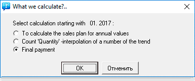

Table of the result of calculation of the "sales plan" for the product N:
| Months | 1 | 2 | 3 | 4 | 5 | 6 | 7 | 8 | 9 | 10 | 11 | 12 |
| 1 year | 60 300 | 54 200 | 48 200 | 67 500 | 50 600 | 50 610 | 50 610 | 50 610 | 75 915 | 88 515 | 101 220 | 113 820 |
| 2 year | 159 060 | 143 110 | 127 270 | 127 270 | 95 370 | 67 048 | 67 048 | 67 048 | 100 572 | 117 392 | 134 212 | 151 032 |
| 3 year | 216 840 | 195 240 | 173 520 | 173 520 | 130 080 | 91 098 | 91 098 | 91 098 | 136 584 | 159 390 | 182 196 | 204 876 |
Sales planning tools in the "Budget-Plan Express" include additional options for price adjustments and forecasting - see "Adjustments to price series using moving averages" and "Sales plan. Models of moving averages".
Calculation Algorithms for Sales Planning "by Yearly Values"
Price calculation algorithm
In the result of the calculation of "by annual values," the price for the beginning of each year is taken as the basis for calculating the price of the trend, according to the formula:
-
Pricen = 1 × Factorn,
Where:
Price n - the price in the n period.
Price 1 - the price at the beginning of the year.
Coefficient n - (percentage of seasonality) / 100 in the n period.
 Permissible fluctuations of seasonal prices can be from -100% to +100%. Seasonality of prices, in fact is deviation from the original number in %.
The algorithm for calculating the quantity
As a result of the calculation of "by annual values," the annual sales volume (quantity) is distributed along a number, depending on the seasonality trend, according to the formula:
-
Quantity n = Quantity year × Coefficient n , where
Coefficient n = Seasonality n / ∑ Seasonality i ,
Where:
Quantity n - quantity in the n-th period.
Quantity year - total annual quantity.
Coefficient n - in the n-th period.

Example of calculating the quantity.
Let the company plan to sell 100 units of production in a year. According to the observations of previous years, seasonal fluctuations for each month, according to a 100-point scale (100%), constitute a trend: Ai = {50, 70, 60, 70, 90, 10, 0, 30, 70, 70, 80, 100}.
- step. Enter the number 100 in the "annual sales -1, 2 and 3 year" fields (in this example, the annual sales volume).
- step. Set the values for seasonality, respectively: 50%, 70%, 60%, 70%, 90%, 10%, 0%, 30%, 70%, 70 %, 80%, 100% . To adjust the values of the sliders, you can use the arrow keys, pre-displaying the seasonality value (mouse hover).
- step. Click the "Calculate" button and select: "Calculate sales plan - by yearly values".
The calculation of the amount shown in the table:
| Planning quantity - value | Jan | Feb | Mar | Apr | May | June | July | Avg | Sen | Oct | Nov | Dec | Total |
| 1.Seasonal trend - on a 100-point scale | 50 | 70 | 60 | 70 | 90 | 10 | 0 | 30 | 70 | 70 | 80 | 100 | 700 |
| 2. Estimated coefficient = Value of row 1 / 700 | 0,07 | 0,10 | 0,09 | 0,10 | 0,13 | 0,01 | 0,00 | 0,04 | 0,10 | 0,10 | 0,11 | 0,15 | 1,00 |
| 3. Quantity = 100 * Value of row 2 | 7 | 10 | 9 | 10 | 13 | 1 | 0 | 4 | 10 | 10 | 11 | 15 | 100 |
Import data. Edit
Planning safety stock of finished products
 Only "actualized" periods are available for editing.
In the table "Remains of finished goods at the beginning of the period" the following values are calculated:
- Price, weighted average (price without VAT)
- Calculation of residuals
- Calculation needs.
Kind of the tab "Accounting for finished products":
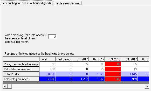
 The result will appear in the table after performing the final calculation: "Data → Calculate → "Sales plan"". Same thing - F9.
Calculation of need
The need for production (purchases) is calculated by the identical formula:
-
Requirement [i] = Sales [i] + (Stocks at the end of the period [i + 1] - Inventories at the beginning of the period [i] ) - Remains of the past period [0] ,
Where i is the period.
Calculation of the weighted average price

To calculate the weighted average is performed step-by-step cyclic algorithm when the weighted average price, calculated in each i-th period, enters into a subsequent period, where is calculated according to the formula:
AP [i] = (Amount of inventory at the beginning[i-1] * Suzana [i-1] + Number of purchases [i] * cost [i]) / (Quantity [i-1] + [i])
Where AP – average price i period.
